Balancing the Inverted Pendulum: An Introduction to Fuzzy Logic Control

TL;DR

• Goal. Balance a rod on a moving cart with rules in plain words, not equations.
• Idea. Fuzzy logic: a value belongs to overlapping terms like “negative small” to a degree, so word rules work on numbers.
• How. Fuzzify the angle and angular velocity, fire 36 rules, take the centroid as the force.
• Result. The rod stays upright in simulation, with no model of the system. An interactive demo shows each stage.

Introduction

With some practice, it’s possible to balance a broom upright in our hand, relying largely on intuition rather than calculation. Yet, the dynamics behind this seemingly simple act are more intricate than they appear. From an engineering perspective, this balancing act is analogous to the inverted pendulum, a classic problem in control theory.

The inverted pendulum is a system consisting of a tall rod, like our broom, but this time, it’s attached to a horizontally moving cart. The objective? Keep the rod upright, compensating for any disturbances that might knock it off balance. A small tilt grows on its own unless the cart moves to catch the rod, because the upright position is unstable. Even so, the system is simple enough to understand and simulate, which makes it a good test bed for a controller.

In the previous post, we derived how the cart and rod respond to a push and tried balancing the rod ourselves. Doing that well meant watching both how far the rod leaned and how fast it was turning, and this time we write that judgement down as rules that decide how to push.

Control theory offers controllers designed from a mathematical model of the cart and rod, including their masses, lengths, and friction. But when we balance a broom, we clearly don’t solve its equations of motion; we react to how far it leans and how fast it falls, in a way we could put into words. This suggests that a controller for the inverted pendulum could be written the same way, as rules in words, without a model of the system.

What if we wanted to introduce an element of that human intuition into our control systems? Enter fuzzy logic, a method that resembles human reasoning by working with concepts that aren’t strictly true or false but lie somewhere in between. Instead of computing directly with the numbers, a fuzzy controller reasons with descriptions like “almost upright” or “slightly tilted.” Its rules only see how well the current state fits those descriptions, so we can write the controller in the same coarse terms we would use to explain balancing to another person. This approach offers flexibility, especially when precise data is unavailable.

Unlike Boolean logic, where a statement is either True or False, fuzzy logic allows degrees of membership between 0 and 1. For instance, describing weather as “0.72 sunny and 0.18 cloudy” provides more information than simply stating “the weather today is sunny but not cloudy.” Those numbers are membership values rather than probabilities, so they need not add up to 1, a distinction Zadeh’s 1965 paper introducing fuzzy sets (PDF) draws between graded membership and statistical uncertainty. With these descriptions, we can construct fuzzy rules, which resemble human thinking and are written as “If … then …” statements. To use them in a machine, we need to give both the descriptions and the rules a mathematical meaning.

Engineers have done exactly that for decades. In the mid-1970s, Mamdani (1974) and Mamdani and Assilian (1975) used fuzzy logic to turn a human operator’s rules for a laboratory steam engine into an automatic controller. By the early 1980s, cement kilns were controlled commercially with linguistic fuzzy rules, and in Japan, fuzzy control then moved into trains and consumer products. When the Namboku Line of the Sendai subway opened in 1987, its trains used a fuzzy controller from Hitachi for accelerating and braking, and Hitachi’s engineers reported better ride comfort, more accurate stops, and lower energy use. Consumer products followed. Canon’s H800 camcorder, released in June 1990, used fuzzy logic for its autofocus, and Hitachi washing machines and Matsushita vacuum cleaners used fuzzy rules to set the wash cycle and suction power from their sensor readings.

Figure 1: The free-body diagram of the cart and rod, adapted from the previous post. The controller chooses the horizontal force \(F\), \(\phi\) measures the tilt from upright, and \(b\dot{x}\) is the damping that opposes a cart moving right. \(N\) and \(P\) are the horizontal and vertical forces at the pivot, which act in opposite directions on the rod and the cart, and \(mg\) is the rod’s weight. Forces on the rod are drawn in teal and forces on the cart in red.

Returning to our inverted pendulum on a cart, the system is shown in Figure 1. The control force \(F\) will depend on the signed angle \(\phi\) from upright and its angular velocity \(\dot{\phi}\). A rod leaning right may be falling farther right or already returning toward upright, so the rules need both inputs. With fuzzy logic, the relationship between these variables becomes linguistic, a much looser form than an equation. That lets us write the rules from common sense, such as “If the pendulum is balanced, then hold very still and apply no force.” In the terms this controller uses, one rule says, “If the angle is positive small and the angular velocity is positive small, then the force is positive small.” How do we turn those words into a force the cart can actually apply?

Fuzzy logic

Our controller receives the angle \(\phi\) in degrees and the angular velocity \(\dot\phi\) in degrees per second, and it returns a force \(F\) in newtons. Zero angle means upright. A positive angle means the rod leans right, a positive angular velocity means it rotates toward the right, and a positive force pushes the cart right. The previous post uses the same convention but calls the angle \(\theta\) and measures it in radians.

Looking at “If … then …” rules like the ones above, a few questions come up. Is “If … then …” an implication in the sense of logic? How can we model labels like “small,” “medium,” and “large”? And with a finite number of rules, how do we handle every numerical input the sensors might measure and turn it into an actual control action? Fuzzy logic answers these questions, and fuzzy control is the practice of building controllers on that mathematics.

As an overview, let’s break down how the fuzzy decision process works step by step. First, fuzzification uses membership functions to assign each numerical input a degree of membership in each linguistic term. The inference phase evaluates the “If … then …” rules and combines their contributions into an output membership function. Finally, defuzzification converts that function into a single numerical force. The full process is illustrated in Figure 2.

Figure 2: Numerical inputs pass through fuzzification, rule inference, and defuzzification to produce a numerical output.

The sections below take these stages in order. Each starts with the general idea, then describes the choices our controller makes and shows the corresponding code. Throughout, we follow one state, a rod tilted \(5^\circ\) to the left and rotating left at \(3^\circ/\mathrm{s}\). The code excerpts come from fuzzy_control.py, where fuzzify, inference, and defuzzify are methods of a FuzzyControl class that runs as a whole.

Fuzzification

One of the distinct advantages of fuzzy logic is that it can process linguistic variables, whose values are words or phrases from natural language rather than numbers. Zadeh proposed them in 1973, together with fuzzy if-then rules relating them, as a way to describe systems too complex or ill-defined for precise mathematical analysis, and developed the idea at length in 1975. In a controller, they are the input and output variables. Typically, a linguistic variable is broken down into a set of linguistic terms, each covering a portion of its values. To describe the rod’s angle, we naturally use terms such as “almost upright,” “slightly tilted,” and “falling over.” For this controller, we decompose the angle into the set {negative big (NB), negative medium (NM), negative small (NS), positive small (PS), positive medium (PM), positive big (PB)}. Each member of this set is called a linguistic term. The angular velocity and the force use the same six names, each with its own range of values.

A membership function \(\mu_A(z)\) quantifies a linguistic term \(A\) by telling us how well a numerical value \(z\) fits it, on a scale from 0 to 1. This answers our second question, how to model labels like “small.” Membership functions appear twice in a fuzzy controller. Fuzzification uses the input terms’ functions to turn numbers into degrees of membership, and defuzzification uses the output terms’ functions to turn degrees of membership back into a number.

Each membership function in our controller is a Gaussian,

\[ \mu(z) = \exp\!\left(-\frac{(z-a)^2}{2\sigma^2}\right). \tag{1}\]

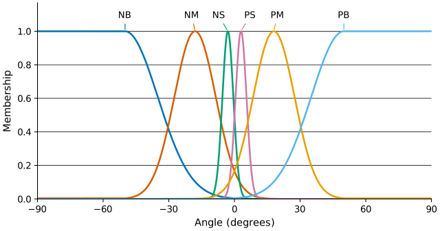
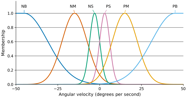
Here, \(a\) is the center of a term, where membership reaches 1, and \(\sigma\) sets its width. Both have the same units as the input \(z\). The code chooses a center and width for each of the six terms for each input, giving the curves in Figure 3 and Figure 4.

Figure 3: Angle memberships. Overlapping terms allow one angle to activate several rules.

Figure 4: Angular-velocity memberships, using the same six terms with different centers and widths.

An important characteristic of fuzzy logic is that a numerical value does not have to be fuzzified using only one membership function. Neighboring curves overlap, so a value can belong to several terms at once, with different degrees of membership. For our state, the negative-small angle term has \(a=-3^\circ\) and \(\sigma=2.5^\circ\), so at \(\phi=-5^\circ\) its membership is about 0.726. The broader negative-medium term gives the same angle a membership of about 0.392. Both descriptions therefore contribute to the rules, rather than the angle being assigned to a single category.

Our simulation knows the angle exactly, so why describe it with vague terms at all? That exactness is a convenience of the simulation. Fuzzy logic is most useful where exact values cannot be observed or stated, and what we know comes from people who describe a situation in words. A patient cannot say how sick they are as a number, but they can say they feel slightly unwell or very ill. A furnace master cannot state the exact properties of the molten metal, yet they describe it in words and decide what to do from that description. Fuzzy rules let a controller use that kind of knowledge directly. The cement kiln controllers from the introduction worked this way, with linguistic control rules that captured the experience of human kiln operators. The point of this toy example is to see whether a controller built the same way, from rules in words and without a model of the cart and rod, can balance the rod. After fuzzification, the rules no longer see the angle itself, only how strongly it fits each of the six descriptions. The code clips the inputs to \([-50,50]^\circ\) and \([-45,45]^\circ/\mathrm{s}\) before evaluating the curves, so every steeper tilt or faster rotation looks the same to the rules. The same clipping flattens the tails in Figure 3 and Figure 4.

In code, fuzzification clips the inputs and evaluates one Gaussian per term. In gaussian, the arguments x, mu, and sig are the input \(z\), the center \(a\), and the width \(\sigma\) from Equation 1.

def gaussian(x, mu=0., sig=1.):
    return np.exp(-np.power(x - mu, 2.) / (2 * np.power(sig, 2.)))


def fuzzify(self, angle, angular_speed):
    angle_memberships = []
    angular_speed_memberships = []
    #
    if angle > 50:
        angle = 50
    if angle < -50:
        angle = -50
    if angular_speed > 45:
        angular_speed = 45
    if angular_speed < -45:
        angular_speed = -45

    angle_mu = [-50., -18., -3., 3., 18., 50.]
    angle_sig = [15., 9.5, 2.5, 2.5, 9.5, 15.]
    for i in range(6):
        angle_memberships.append(gaussian(angle, angle_mu[i], sig=angle_sig[i]))

    angular_speed_mu = [-45., -15., -3., 3., 15., 45.]
    angular_speed_sig = [14., 7.5, 3., 3., 7.5, 14.]
    for i in range(6):
        angular_speed_memberships.append(gaussian(angular_speed, angular_speed_mu[i], sig=angular_speed_sig[i]))
    return angle_memberships, angular_speed_memberships

Rules and inference

Within a fuzzy logic system, a rule base is constructed to control the output variable. A fuzzy rule is a simple IF-THEN rule with a condition and a conclusion. In our controller, each rule’s condition combines an angle term and an angular-velocity term, and its conclusion names a force term. Rule bases like this have a long history in classical AI, where expert systems stored a specialist’s knowledge as “if … then …” rules. Fuzzy control lets such rules work with conditions that hold to a degree, instead of only true or false.

The rules follow what we do with a broom: move the cart toward the side the rod is falling, and push harder the further it leans and the faster it falls. Using our linguistic terms, we construct the rule base below. Rows describe the angle, columns describe angular velocity, and each cell names the output force term.

\(\phi \backslash \dot{\phi}\)	NB	NM	NS	PS	PM	PB
NB	NB	NB	NB	NM	NS	PS
NM	NB	NB	NM	NS	PS	PS
NS	NB	NM	NS	PS	PS	PM
PS	NM	NS	NS	PS	PM	PB
PM	NS	NS	PS	PM	PB	PB
PB	NS	PS	PM	PB	PB	PB

For example, the first cell reads, “If angle is NB and angular velocity is NB, then control force is NB.” If the rod leans slightly right while swinging strongly left, it is already falling to the left, so the PS row calls for NM, a moderate push to the left that brings the cart under the rod before it overshoots. The same lean while swinging strongly right calls for PB.

To evaluate these rules, we need fuzzy versions of AND and OR. Unlike in conventional Boolean algebra, we can choose different operators for intermediate membership values, as long as they give the usual results at 0 and 1. Let \(\mu_A\) and \(\mu_B\) represent the membership functions for fuzzy sets \(A\) and \(B\). The table below lists common choices for the OR and AND operators.

OR (union)	\(\mu_{A \cup B}(z)\)	AND (intersection)	\(\mu_{A \cap B}(z)\)
Maximum	\(\max\{\mu_A(z), \mu_B(z)\}\)	Minimum	\(\min\{\mu_A(z), \mu_B(z)\}\)
Algebraic sum	\(\mu_A(z) + \mu_B(z) - \mu_A(z)\,\mu_B(z)\)	Algebraic product	\(\mu_A(z)\,\mu_B(z)\)
Bounded sum	\(\min\{1, \mu_A(z) + \mu_B(z)\}\)	Bounded difference	\(\max\{0, \mu_A(z) + \mu_B(z) - 1\}\)

A rule in our controller activates only as strongly as its weaker condition, so it uses the minimum for AND. For our state, the angular velocity of \(-3^\circ/\mathrm{s}\) sits exactly at the center of the NS angular-velocity term, so that membership is 1. The NS/NS rule therefore activates at \(\min(0.726,1)=0.726\) and contributes to the NS force term. The NM/NS rule also activates, at about 0.392, and contributes to NM force. Several other rules activate more weakly, and when two rules name the same force term, the term keeps the larger activation.

We now need to give those force terms a numerical shape. Their Gaussian membership functions have centers at \(-30,-20,-10,10,20,30\) N, respectively, and all use \(\sigma=2\) N. Each curve is clipped at its term’s activation by taking the minimum of the two, so an activation of 0.726 caps the NS curve at that height.

Combining the clipped curves into one output membership function is a step called accumulation. Our controller takes the maximum at each possible force, the usual choice, so any active rule contributes without overlapping memberships being added together. The bounded sum from the OR table is another option. It adds the contributions and caps them at 1, so several moderately active rules can together outweigh a single strong one. The normalized sum also adds them but rescales the result so that it stays within 1. The minimum for AND and the maximum for accumulation are the operations used in Mamdani fuzzy inference.

This also answers our first question. In classical logic, “if A then B” is true whenever A is false, so a rule whose condition does not fit the current state would still count as satisfied. Our controller does not treat a rule as an implication in that sense. It clips the conclusion with the minimum, which behaves like AND, so a rule whose condition does not fit contributes nothing to the output. Fuzzy logic does define implication operators that generalize the classical one, but this kind of controller does not need them.

The operators become three small functions.

def fuzzy_or(a, b, type="max"):
    if type == "max":
        return np.fmax(a, b)


def fuzzy_or_array(a, type="max"):
    if type == "max":
        return np.max(a, axis=0)


def fuzzy_and(a, b, type="min"):
    if type == "min":
        return np.fmin(a, b)

inference applies them in the order just described.

def inference(self, angle_memberships, angular_speed_membership):
    #
    # How to interpret the rule base:
    # NB: negative big, NM: negative medium, NS: negative small
    # PB: positive big, PM: positive medium, PS: positive small
    # The table:
    #    NB, NM, NS, PS, PM, PB angular speed
    # NB  0   0   0   1   2   3
    # NM  0   0   1   2   3   3
    # NS  0   1   2   3   3   4
    # PS  1   2   2   3   4   5
    # PM  2   2   3   4   5   5
    # PB  2   3   4   5   5   5
    # angle
    #
    # One cell contains the control force:
    # 0 NB, 1 NM, 2 NS, 3 PS, 4 PM, 5 PB
    rule_base = [[0, 0, 0, 1, 2, 3],
                 [0, 0, 1, 2, 3, 3],
                 [0, 1, 2, 3, 3, 4],
                 [1, 2, 2, 3, 4, 5],
                 [2, 2, 3, 4, 5, 5],
                 [2, 3, 4, 5, 5, 5]]

    fuzzy_control_force = [0., 0., 0., 0., 0., 0.]
    for i in range(6):
        for k in range(6):
            # AND joins the two conditions; OR combines rules for a force term.
            pt = fuzzy_and(angle_memberships[i], angular_speed_membership[k])
            fuzzy_control_force[rule_base[i][k]] = fuzzy_or(fuzzy_control_force[rule_base[i][k]], pt)

    for i, mu in enumerate([h * 10 for h in [-3, -2., -1., 1., 2., 3]]):
        fuzzy_control_force[i] = fuzzy_and(gaussian(self.sample_points, mu, sig=2.), fuzzy_control_force[i])
    fuzzy_control_force = fuzzy_or_array(np.asarray(fuzzy_control_force))
    return fuzzy_control_force

Defuzzification

Following inference, we have a membership value for each possible output force, but the cart needs one force to apply. In Figure 5, the shaded regions represent the fuzzy output, and the arrow marks the single value obtained by defuzzification. One way to choose that value is the center of gravity, or centroid, of the combined area.

Figure 5: Defuzzification turns a combined output membership function into a single value. This is a schematic, and our controller uses Gaussian output curves.

If \(\mu(u)\) is the combined output membership at force \(u\), and \(u_{\min}\) and \(u_{\max}\) bound the output range, the centroid is

\[ F = \frac{\int_{u_{\min}}^{u_{\max}} u\,\mu(u)\,du} {\int_{u_{\min}}^{u_{\max}} \mu(u)\,du}. \tag{2}\]

For equally spaced force samples \(u_i\), we approximate it by the weighted average

\[ F \approx \frac{\sum_{i=1}^{n} u_i\,\mu(u_i)}{\sum_{i=1}^{n} \mu(u_i)}. \tag{3}\]

Each sampled force is weighted by the height of the combined curve there. Other defuzzification methods pick the force that splits the area under the curve in half (the bisector) or average the forces where the curve is highest (the mean of maxima), and they can give different forces for the same fuzzy output.

Our code uses this sampled centroid, with 50 equally spaced forces from \(-30\) to \(30\) N. Because the whole clipped shapes enter the sum, the widths of the output curves affect the force, not only their six centers.

def defuzzify(self, fuzzy_control_force):
    rv = (np.sum(self.sample_points * fuzzy_control_force) + 1e-8) / (np.sum(fuzzy_control_force) + 1e-8)
    return rv

For our state, the NS curve, clipped at 0.726 and centered at \(-10\) N, carries about 41% of the weight in Equation 3. NM and NB add about 39% at \(-20\) and \(-30\) N and pull the result left, while PS, PM, and PB add about 20% between \(10\) and \(30\) N and pull it right. The two pulls nearly cancel, so the force ends up close to the NS center. Running all three stages confirms a force of \(-10.009\) N, pushing the cart left.

controller = FuzzyControl()
angle_memberships, speed_memberships = controller.fuzzify(-5., -3.)
force_memberships = controller.inference(angle_memberships, speed_memberships)
force = controller.defuzzify(force_memberships)
print(f"Control force: {force:.3f} N")

Control force: -10.009 N

This also answers our last question. Because neighboring membership functions overlap, every input activates some rules, and defuzzification turns their combined output into a single force. Six terms per input and 36 rules are enough to cover every angle and angular velocity. The common-sense rule from the introduction, to apply no force when the pendulum is balanced, has no cell of its own, because no term is centered on zero. When the rod is upright and still, the negative-small and positive-small terms activate equally, and their pulls cancel in the centroid, so the force is zero.

Putting it all together

So far, the controller only turns one state into one force. To see whether its rules actually balance anything, we connect it to the cart-and-rod model from the previous post. At every step, the simulation runs the three fuzzy stages on the rod’s current tilt and angular velocity and applies the resulting force. That post derives the equations of motion, and fuzzy_control.py contains the same model next to the controller.

The simulation below runs this loop in the browser and draws each fuzzy stage for the current state. It starts paused at our worked example, so the rule table and the centroid show the same activations and force we computed above. Dragging the angle slider through zero shows NS handing over to PS. Near upright both terms stay active, so the force changes smoothly instead of jumping from one rule to the next. Once the simulation runs, pushing the cart makes the rod swing the other way, and the output curve’s weight shifts to push back. Switching the controller off shows how quickly the rod falls on its own.

We started with a broom balanced on a hand, kept up by intuition rather than calculation. Thirty-six rules, each a sentence we could say out loud, now do the same for a rod on a cart, and the controller never solves the equations of motion. The cart drifts as it works, because the rules only describe the rod, and rules about the cart would be the natural next step.

Citation

Cited as:

Englert, Brunó B. (July 29, 2023). Balancing the Inverted Pendulum: An Introduction to Fuzzy Logic Control. englert.ai.

Or

@misc{englert2023fuzzy,
  title        = {Balancing the Inverted Pendulum: An Introduction to Fuzzy Logic Control},
  author       = {Englert, Brunó B.},
  howpublished = {englert.ai},
  year         = {2023},
  month        = {July},
  url          = {https://englert.ai/posts/002_fuzzy_control/englert_ai_2_fuzzy_control.html}
}

Source code

The Python files need NumPy, and the desktop animation also needs Arcade 3. The command below installs both.

python -m pip install numpy arcade

• fuzzy_control.py contains the complete controller, the cart-and-rod model, the worked example, and a 10 s closed-loop run. Run it with python fuzzy_control.py.
• arcade_simulation.py is a desktop animation built on fuzzy_control.py. Hold the arrow keys to push the cart with 10 N, press Enter to switch the controller off and on, R to reset, and Space to save a screenshot.